Circular slide rules

Introduction

Although circular slide rules have some advantages over linear slide rules they were never as popular. The two main advantages of this type of slide rule are:

• They are more compact. A scale of 10 cm diameter has a length 30 cm.
• While calculating with a linear slide rules having a basic range of scales there is sometimes a need to switch the index. This is never necessary with circular rules. Some linear rules had special scales (e.g. CF and DF folded scales) to avoid having to do this; these special scales are unnecessary on circular rules.

For many users these advantages were offset by the fact that scales near to the centre of a rule had less accuracy than scales near the edge and it is necessary to keep on turning the rule (unless the user gets good at reading scales upside-down and sideways!).

Although many companies made circular rules, and they look different (e.g. flat plastic, pocket-watch types etc.), in fact there are only two types of rule: those with two disks and a single cursor and those with a single disk and two cursors. Among the former are rules by Concise and Fearns; among the latter are rules by Gilson and Fowler. In these instruction I deal with rules of both types pointing out special features of individual models such as the the "binary" scale on the Gilson rules or the spiral scale on the Fowler.

Rules with two disks and one cursor

Makers and construction

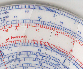
This is the commonest type of circular rule. Rules of this type were made by Concise, Aristo and Fearns. With some of them there were two disks, the outer one being rebated to take the inner one. With others there was a flat circle (very much the equivalent of the slide of a linear rule) with static disks outside and inside it.  In many cases the disks were protected by a flat sheet of clear plastic; this did have the disadvantage of introducing  more possibility of errors in reading the scales due to parallax. Examples of sub-types are given below.

The examples for this type of rule are given using a Concise 300B. This rule has the advantage that the scales are labelled as A, B, C etc. and the index (i.e. 1) is clearly marked. The cursor is also labelled with the names of the scales which makes reading scales easier at intermediate points. It is also a duplex rule with a wide range of scales which means that it can used to describe the way to use many other rules.

Front view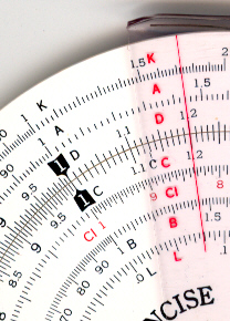

Back view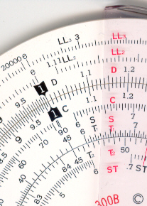

C and D scales

As with linear rules, these are the scales most used for basic calculations and the way to multiply and divide on circular rules is very similar to using linear slide rules. We'll start first with simple multiplication and division and then consider calculations with several factors and divisors.

Simple multiplication

Calculation: a * b
    1.0 on C to a on D
    Cursor to b on C
    Answer under cursor on D.

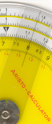
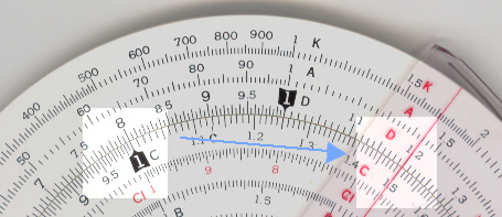
Example: 8.0 * 1.5     1.0 on C to 8 on D     Cursor to 1.5     Answer (12.0) under cursor on D.

Simple division

Calculation: a / b
   Cursor to a on D
    b on C to cursor
    Answer on D against 1 on C

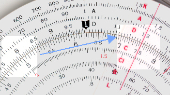
Example: 1.4 / 7     Cursor to 1.4 on D     7 on C to cursor     Answer (0.2) on D against 1 on C.

Combined multipliation and division

Calculation: a * b / c
   Cursor to a on D
    c on C to Cursor
    Cursor to b on C
    Answer on D under cursor.

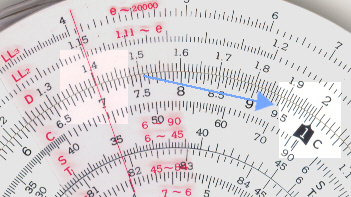
Example: 8 * 7.5  / 5     Cursor to 8 on D     5 on C to cursor     Cursor to 7.5 on C.      Answer (12) on D under cursor.

If there are further pairs of multiplication and division you can extend the above calculation indefinitely. To extend the above by multiplying by d and dividing by e.

Calculation: a * b * d / ( c * e )
   Cursor to a on D
    c on C to Cursor
    Cursor to b on C
    e on C to Cursor
    Cursor to d on C
    Answer on D under cursor.

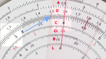
The following example is an extension of the one above. Example: 8 * 7.5 * 4 / ( 5 * 3 )     Cursor to 8 on D     5 on C to cursor     Cursor to 7.5 on C.     3 on C to cursor     Cursor to 4 on C.      Answer (16) on D under cursor.

The above method works best when the number of numerators is 1 more than the number or denominators. However it is possible to re-arrange an expression by using extra 1s. For example:
    (a * b * c * d) / (e * f )

can be re-written as:
    (a * b * c * d) / (e * f * 1 ) .

Similarly:
    (a * b ) /( c * d * e * f   ) .

can be re-written as:
    (a * b * 1 * 1 * 1 ) /( c * d * e * f  ) .

This may appear at first to complicate the calculation but in fact no extra movements are needed.